We want to generate data that will be consumed by computers, not humans. There are two ways to produce biological data at the scale required for this, and we’re thinking deeply about both:

1. Maximize the number of datapoints you generate per experiment.
   We’ve been tackling this through an “O(1)” experimental approach, covered in a prior post.
2. Minimize the latency of each experiment.
   This is our focus in this post. An experiment’s “latency” is how long it takes to get from a design on the computer to data. It happens via the complicated, annoying, and messy physical world of data collection.

When the experiment itself is slow and complicated, you’re limited in how many times you can iterate. That means that for anyone building a “lab-in-the-loop,” experimental latency becomes the primary bottleneck. Brute-forcing throughput with automation can add more inertia — you have to commit to a design way in advance and then wait for the entire campaign to run, sacrificing the ability to pivot and stretching your iteration cycle. We think there are more nimble, elegant solutions to pursue.

As we have in previous posts, we’re going to try to solve this experimental problem by adapting tools and language from computer science; in this case, clean coding norms. Coders know good code when they see it. Or rather, when they smell it; code smell is a subtle sign that something is wrong with a piece of code. It isn’t a bug, but developers learn to sense that it will be hard to change or likely to break.

And one of the most recognizable of such signals is spaghetti. It’s poorly structured, tangled, and full of weird dependencies. Spaghetti code is hard to debug and maintain, and it’s pernicious — spaghetti begets more spaghetti. On the other hand, clean code is, well, clean. It’s easy to read and trace how inputs and outputs relate, it runs deterministically (a given input always results in the same output), and most importantly of all, it’s easy to debug and maintain. Clean code is typically built from functions — self-contained units that take in well-defined inputs and deterministically return well-defined outputs. Each function is easy to understand, test and, importantly, swap out independently of any code around it.

We’ve found that experimental genomics has some similarities. We want reliable processes that can be prototyped quickly and provide deterministic data, but we often end up with spaghetti protocols that are bloated, complex, and non-modular. In fact, our company ended up in a place like this and it almost killed our experimental work. Here’s how we defused that by making a number of deliberate, CS-inspired decisions that made our lab workflows run like clean code.

Applying good coding practices to genomics

Imperative instructions obscure the logic underlying a workflow

Genomics protocols typically read like a series of commands: “get this tube,” “add this to the tube,” “heat the tube up,” and so on. In coding, such a structure resembles imperative programming, an approach that has the potential for all sorts of issues.

Let’s examine a pretty standard small-RNA-seq workflow, a class of protocols that we’ve spent a good amount of time working on in the past. At a very high level, the process takes a set of input RNAs (“inserts”), adds sequence handles (5′ and 3′ adaptors) that DNA sequencers expect, converts the RNAs into DNA (“reverse transcription”), and exponentially amplifies this material (“PCR amplification”). Along the way there are also a whole host of side-processes (kinase this, dephosphorylate that, destroy this, and so on).

Here’s a schematic of the entire process (don’t get too bogged down in the details, we’ll just talk about specific aspects of this):

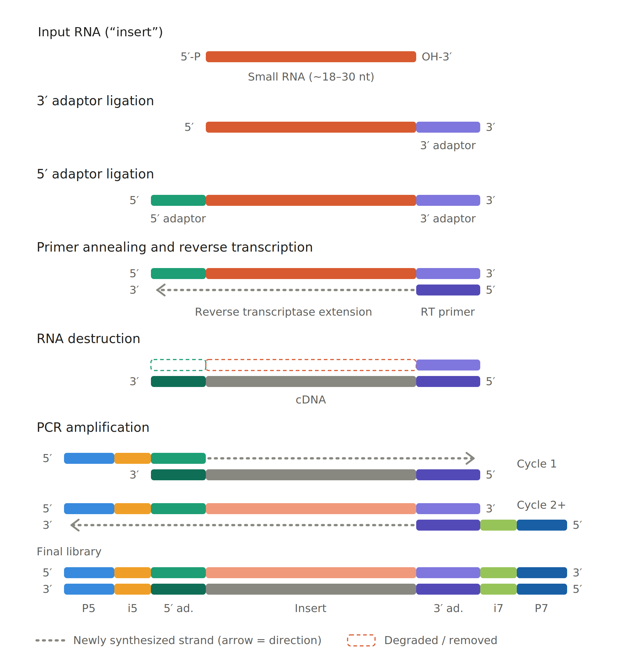
One phase of this process — RNA destruction — can serve as a pretty nice example of what goes wrong with imperative protocols. Imagine a scientist wants to deploy this method and finds a few basic protocols online. They mix and match steps based on what seems easiest to accomplish in the lab with the reagents they have. They get to the point where they need to degrade just the RNA from a mix of RNA and DNA. A cheap and easy way to do this is to simply increase the pH. The scientist implements this and then proceeds to the final PCR amplification step. Uh oh, it fails. Why?

In pseudocode form, their imperative protocol might look like this:

PH: float
FRAGMENTS: list[dna | rna]

def main():
    global PH
    PH = set_pH(7.5) # neutral pH
    destroy_rna()
    pcr_amplify()

def destroy_rna():
    """
    uses alkaline hydrolysis to destroy RNA but not DNA
    """
    global PH, FRAGMENTS
    PH = set_pH(10.5)
    FRAGMENTS = [f for f in FRAGMENTS if not is_rna(f)]

def pcr_amplify():
    global FRAGMENTS
    if PH > 8.5:
        FRAGMENTS = FRAGMENTS
        # PCR enzyme is not active at high pH, no amplification
    else:
        FRAGMENTS *= 2**20
        # 2^20 amplification from 20 cycles of PCR amplification 

main()

Programmers might look at this code block and realize that there’s something weird going on. For the non-coders: there’s a global state variable (pH) that was explicitly set at 7.5 (because the scientist prepared standard buffers with neutral pH for the ligation steps at the start of the workflow). Yet during the course of the experiment, an intermediate process changed the pH state in a way that was invisible (molecular biology is famously clear liquids all the way down). The scientist was thinking one step at a time, and didn’t consider how increasing the pH to destroy RNA would affect the final PCR amplification. The PCR enzyme didn’t work at high pH, so the run failed.

This is the equivalent of code with mutable global variables, and such code is really hard to work with. It’s difficult to isolate bugs or repurpose this type of code, and most problematically, it makes it impossible to reason locally. One can’t just inspect pcr_amplify and understand what will happen; they’d have to know the full process history of the workflow. Nothing can be tested in isolation, interchangeable modules can’t be swapped out for each other, and so on.

Sounds terrible, right? Fear not — computer science can help us.

Making genomics function-al

Let’s apply the principles of functional programming to genomics.

How would a coder fix our pH problem? One solution would be to reset the global state between every step, perhaps something like this:

def main():
    global PH
    PH = set_pH(7.5)
    destroy_rna()
    PH = set_pH(7.5)
    pcr_amplify()

This might feel reasonable to an experimentalist too: it’s the logic of the “with-bead” genomics prep from Fisher et al. They have a multi-step genomics workflow, and to sidestep issues arising from reagent carryover, they explicitly purify their DNA library at every step and put it back into neutral buffer (i.e., resetting the global pH variable).

But let’s think a little deeper. A programmer doesn’t want to manually reset the global state a bunch of times, and an experimentalist doesn’t want to deal with several DNA bead purifications if they don’t have to. A simpler solution would be to prevent processes from ever changing the global state at all. As we’ve alluded, this is the idea behind pure functions: they carry out some process deterministically and reproducibly without any side effects that could affect other downstream processes.

So instead of changing pH to destroy RNA, we need to find an alternative that doesn’t change the global state — perhaps an enzyme like RNaseH that chops up RNA at neutral pH and doesn’t interfere with PCR. With this simple adjustment, everything is carried out in the same buffer, with no step-to-step coddling. The solution, in pseudocode, is simple:

def destroy_rna(fragments: list):
    """
    uses RNase enzymes to destroy RNA but not DNA
    """
    product = [f for f in fragments if not is_rna(f)]
    return product

While an enzymatic solution isn’t always an option (some enzymes are very finicky about what’s in their reaction), there are enough useful enzymes with interoperable requirements (like these) that you can get very far when you apply this type of simplification to genomics workflows.

Extending the metaphor

Readable code makes its logic and structure apparent — not by explaining every line in comments, but because the steps fit together coherently. Expressing experimental protocols this way (instead of “do this,” “do that”) makes them easier to grasp and remix.

For example, here’s a more complete pseudocode picture of the workflow schematized above:

adaptor_5p: dna = "ACGCTCTTCCGATCT"
adaptor_3p: dna = "GATCGGAAGAGCACA"

def ligate_5p(insert: rna):
    product = adaptor_5p + kinase_5p(insert)
    return product

def ligate_3p(insert: rna):
    product = dephosphorylate_3p(insert) + adaptor_3p
    return product

def reverse_transcribe(ligated: rna):
    if adaptor_3p not in ligated:
        return None
    product = dna(reverse_complement(ligated))
    return product

def destroy_rna(fragments: list):
    """
    uses RNase enzymes to destroy RNA but not DNA
    """
    product = [f for f in fragments if not is_rna(f)]
    return product

def amplify(template):
    if is_rna(template):
        return None
    if adaptor_5p not in template or adaptor_3p not in template:
        return None
    return template * 2**20

What makes this more intuitive than an imperative protocol would be? One benefit is that biological processes that work in tandem to accomplish a goal are grouped together instead of appearing as separate steps with no obvious connection. For example, you need to treat the RNA fragments (“inserts”) with a 5′ kinase for the 5′ adaptor ligation to work (this is a bit hard to read, but 5′ is just a way to refer to a specific end of a piece of RNA or DNA — not super relevant to the point we're making). Describing steps of the workflow like we have above makes it easy for the reader to figure out what’s happening: the 5′ kinase and 5′ ligase steps are grouped because they together carry out a single function [[1]]. A reader faced with a typical protocol must understand the entire process before this is clear. In pseudocode, it’s immediately apparent.

A function-like representation is also a good way to help someone easily comprehend the full workflow at a high level. For example, the following abstraction would allow a reader familiar with code to quickly grasp the order and dependencies of a protocol without getting bogged down in arcana like “T4 RNA Ligase K224Q” or whatever:

amplify(
    destroy_rna(
        reverse_transcribe(
            ligate_5p(
                ligate_3p(insert)
            )
        )
    )
)

When we represent genomics processes as functions, we can borrow other helpful CS concepts too. For example, some genomics processes are order-independent or “commutative” (you can do them in any order with the same outcome), while others aren’t. Establishing these rules explicitly makes caveats clear early on and gives you flexibility in how you design a full process. Here’s an example:

ligate_3p(ligate_5p(insert)) == ligate_5p(ligate_3p(insert))
    True
    
ligate_3p(reverse_transcribe(insert)) == reverse_transcribe(ligate_3p(insert))
    False

There are other fun, useful parallels between CS and genomics, but we’ll wrap the theoretical part of this post up here. Thinking of (and even representing) physical wet-lab processes like code can provide a structure that spotlights critical information and makes protocol design easier, modular, and more flexible[[2]].

We’re not suggesting all biologists need to start writing in pseudocode, but we’d love to experiment with more intuitive protocol formats and encourage others to do so as well. The "methods paper" as we know it could use a refresh — there must be a better way to spell out the logic behind each choice instead of focusing on the outcome. We don't have all the answers, but hope to spark conversation on this front.

Next, we’ll show you how we applied these concepts in the real world, to save our most important workflow when it was circling the drain.

Untangling spaghetti genomics

Functional programming has been a useful framing device so far, but its true power is apparent when applied to complex, tangled protocols. Real-world workflows aren’t nearly as tidy as our toy example above. Big, multi-step genomics processes tend to start off looking nice on paper, and sooner or later become a bloaty mess. For example, about a year ago, our protein-interaction workflow looked pretty nightmarish:

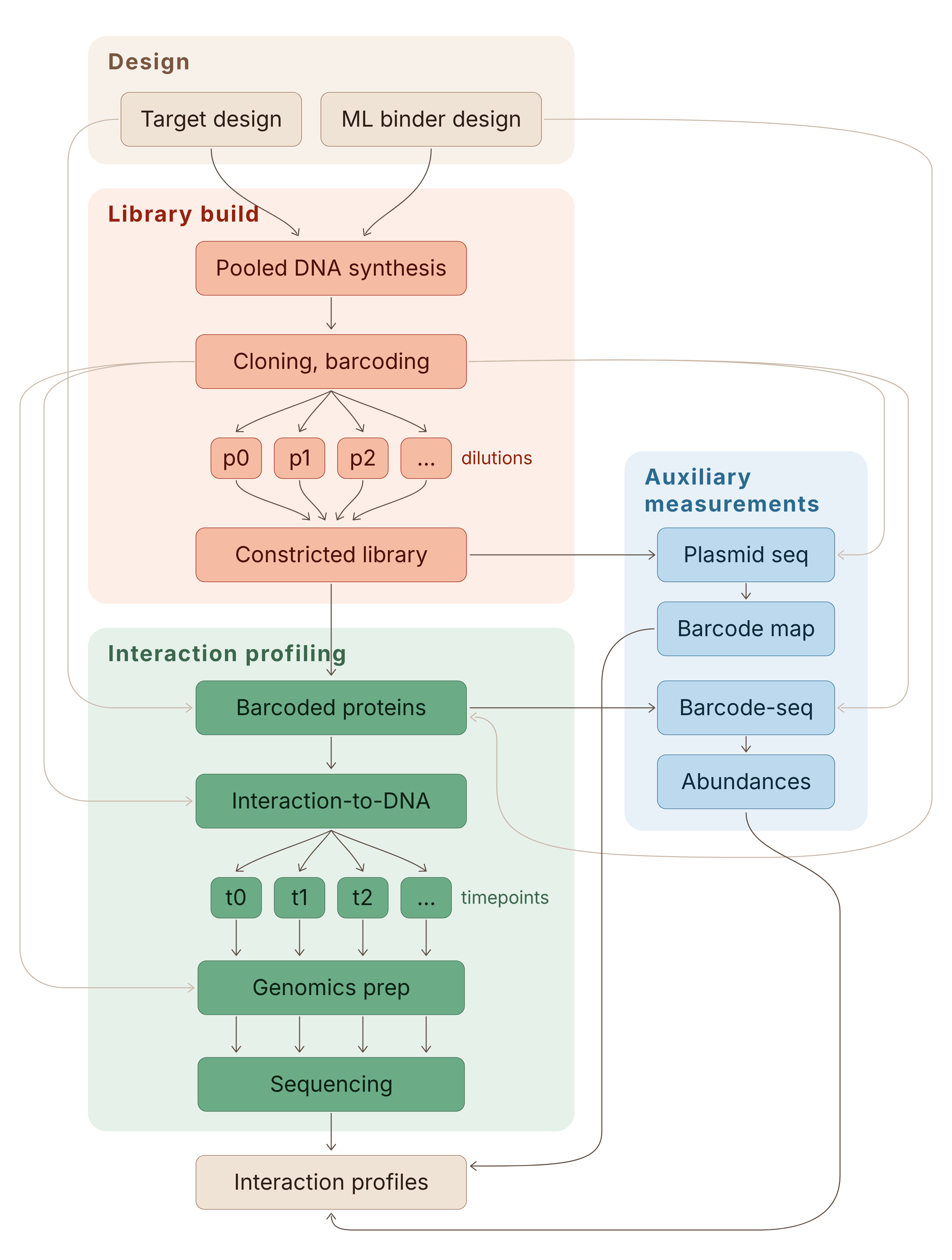
To a programmer, this is spaghetti code. While there’s one primary input (i.e., lists of protein sequences) and one primary output (protein–protein interaction data), there’s a huge mess in the middle. Among the slew of intermediates are tubes that get QC’d, others that get sequenced, and yet others that are not tubes at all, but digital outputs, and so on.

Even if this worked (and honestly it hardly did), it was completely unmaintainable. When we tried to make one tiny change — say, a different primer — we had to trace how that change’s effect propagated through a million places, and inevitably we’d forget something, or something unexpected would happen. Then we’d sit there debugging and fiddling and generally not getting very much done. So as you’d expect, improving our system was horrendous and slow.

To get to where we are now, we had to fully refactor this. We started conceptualizing the workflow as code, and looked for opportunities to tighten it up. We trimmed down the workflow, removed weird branches and cycles, and compartmentalized the various parts. In other words, we added clean coding norms to genomics.

While there are still a couple of rough edges, the workflow has been substantially pruned. There’s no multi-branching “fans,” no paths that generate auxiliary inputs that need to be kept track of, everything is (almost) a nice, clean, linear flow.

Simplification #1: Eliminate experimental randomness

Biology itself is inherently quite random. And though our overall assay setup isn’t complicated by any actual biology (for now!), we found that our workflows exhibited nondeterministic behavior that made maintaining and debugging the workflow complex and frustrating.

Where does that randomness come from? A little background: A common part of many genomics workflows like ours is to assign a DNA barcode to a protein variant so you can later track it with DNA sequencing. In a nutshell, the standard way to do this is to randomly combine a set of variant-encoding DNA (“libraries”) and information-encoding DNA (“barcodes”) together, and then introduce them into bacteria. Each resulting bacterial cell then clonally propagates into a colony that (ideally) carries a single variant + barcode pair. You then move forward by picking enough of those colonies to be sure you’ve captured your whole library of variants.

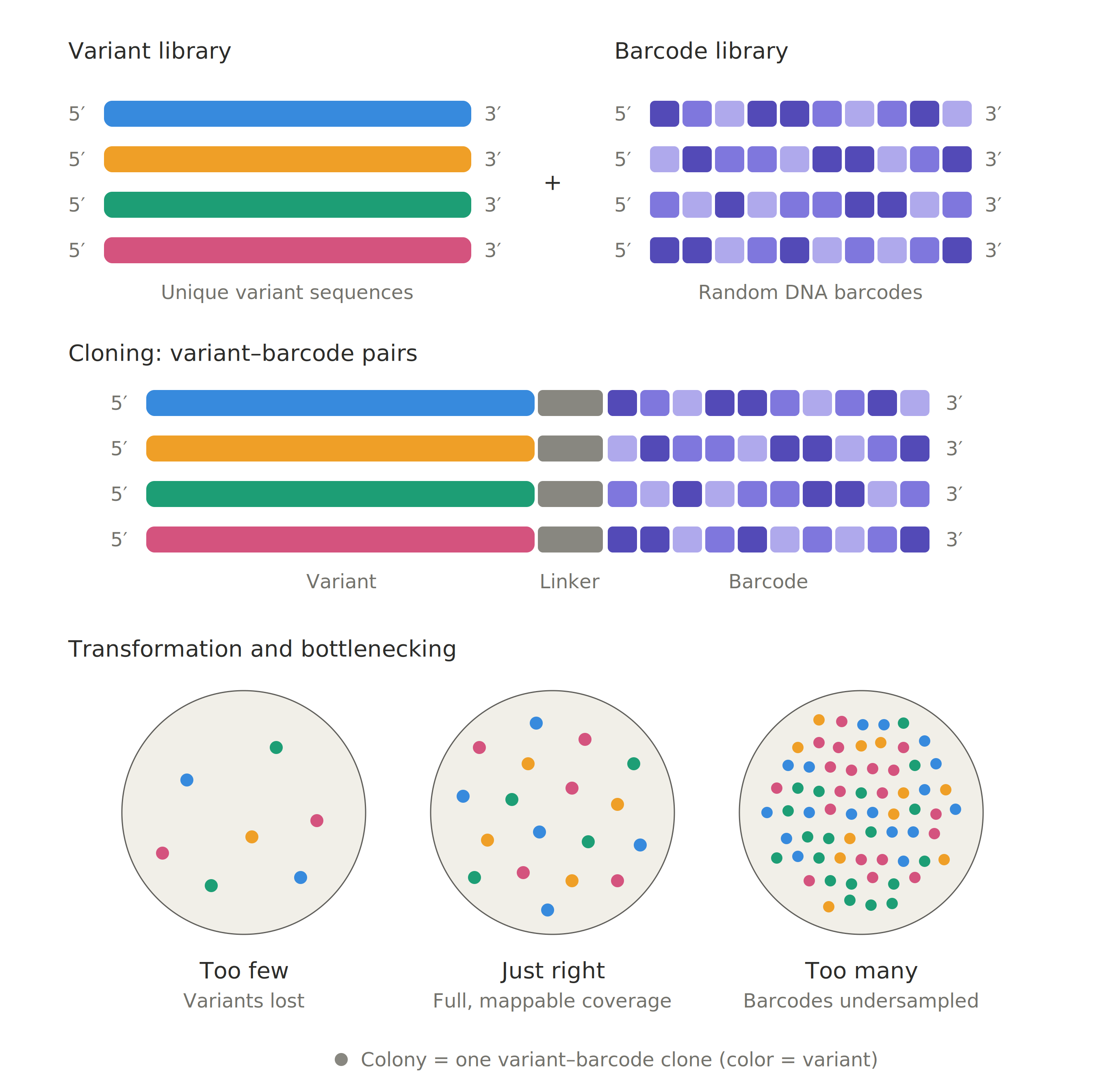
PROBLEM: The first issue is that there’s a “Goldilocks zone.” Imagine you designed 1,000 protein variants, but only end up with 200 colonies — you’re obviously missing a ton of variants. What if you end up with 200,000 colonies? The same barcode will be attached to several different protein variants, making it impossible to use the barcode to track each protein variant accurately. We found that identifying the sweet-spot of colony count was fragile and frustrating — it meant making dilution plates, counting colonies, scraping plates, and generally doing a bunch of annoying labwork.

PROBLEM: It gets even worse. Let’s look at this like a software engineer might: this is a process (variant barcoding) that’s in the middle of a very complex workflow and whose output is random (i.e., each protein variant gets randomly assigned a barcode). There’s no way to set a seed to make it run deterministically, and the output is very very hard to inspect, version-control, or checksum[[3]].

Clearly there’s no salvaging this, it’s gotta go.

SOLUTION: We realized that we could encode each barcode and protein variant pair within a single oligo (at the cost of more expensive DNAs). The labor cost is lower and there’s no longer any random behavior because the barcode-to-variant mapping is fixed at the DNA design stage. With this change, our process became way simpler (there’s no need to run a side sequencing process) and the data became cleaner:

Why haven’t we always treated biology this way?

If we run code on a given input, we expect the outputs to be exactly the same every time. We demand absolute reproducibility from algorithms and software.

So why is biology held to a different standard? Well, because it’s biology. Living things work in a way that’s muddy and stochastic[[5]]. At the molecular level, no two cells are equivalent[[6]]. Even if you had the world’s most reliable protocol, you couldn’t truly reproduce an output because the inputs will never be the same.

Thus, we don’t treat biology itself like code, but we’ve seen major benefits from applying programming principles to the process of studying biology. This framing — approaching biology as an engineering discipline — wasn’t really possible until recently. And it’s not because biology exists in the physical world — hardware is physical too, and hardware engineers have been building reproducible systems and methods for decades. So what’s different?

Hardware engineering is cumulative because it’s built from self-contained building blocks, or components, that follow shared standards: to use one in your own device, you only need to know its specs. Fields like electronics work this way because practitioners can measure their components’ properties well (think voltage, memory capacity, or bandwidth). Software engineering doesn’t quite interact with the physical world in the same way, but it convergently evolved a similar ruleset that enables modularity — clean code norms with functions, modules, APIs and the like. A component is a physical object whose properties you can specify, while a function is a process whose inputs and outputs you can specify.

Biology has both but specifies neither — there’s rarely anything like a datasheet. We think this is for two main reasons: first, biology is difficult to measure, and second, biology’s components (e.g., oligos and enzymes) and functions (e.g., ligation, amplification, sequencing) are typically very context-dependent[[7]]. Specifying biology ultimately requires measuring components and functions across every context they may be used in, or building models that can extend measurements from one context to another. Until recently, neither was practical — measuring across contexts was either impossible or prohibitively expensive, and models that could bridge contexts simply didn’t exist.

So why do we think this is doable now? Cheap DNA synthesis lets us take a “shotgun” approach toward experimental variables and parameters, cheap sequencing lets us measure all of this (even if it’s likely that many of these conditions are going to be low-information), and cheap compute (along with advances in ML) lets us handle this firehose of data and build models that infer between contexts. Together, that changes which tradeoffs are worth making. Every change we made in our assay leans on this: we paid for longer oligos to fix barcoding issues, replaced some auxiliary measurements with experimental and inference complexity, and turned timepoints into barcodes. None of these tradeoffs would have been feasible a decade ago.

Building measured, specified components and functions for genomics assays is one way we can start actually making biology engineerable. When biology gets well-specified parts, they compound[[8]], but unfortunately, protein science has mostly missed out on this[[9]]. One of the goals of our tech stack is to change that — we’re turning protein interactions into DNA, which a well-specified function (DNA sequencing) can read out, so we can mix and match PPIs like everything else. And beyond that, we’re using that protein-to-DNA operation itself as a function that we can build on even further.

Modernizing the wet-lab in the era of AI

To summarize, we think biology protocols are a bit like embarrassing code. If we want to make wet-lab work sufficiently scalable for labs-in-the-loop to succeed, we have to start treating workflows with good coding hygiene. Processes need to be maintainable, with clear norms and structure that make them easy to remix, iterate on, and share between groups.

We’ve experienced the concrete impact of applying a more strategic framework to wet-lab methodology — it helped save our company’s most critical workflow from dying of bloat. Now we apply this thinking to everything we do.

In our view, spaghetti workflows are one of the many reasons why development cycles in experimental biology are so slow. In the lab-in-the-loop setting that we (and many others) are building toward, slow and messy steps compound, lowering the number of “loops” and limiting how “optimal” the output can be.

Taking this a step further, we envision that the processes we’re building will themselves be valuable inputs for a model to ingest. We imagine that at some point, an LLM could design experimental workflows better than a group of puny humans. Right now they don’t, but why? Our best guess is by analogy: if you train a model exclusively on spaghetti code, you’ll generate a lot of bad code. For LLMs to create truly useful and innovative experimental processes, they need to train on a corpus of clean, tidy experimental code. This is exacerbated because, at least to us, the intent of a process is not adequately captured by the imperative style of experimental protocols. (And strapping a camera to a lab tech’s head to track what they’re doing probably won’t help.) Not helping the reader (or the LLM) see why steps are organized the way they are makes genomics seem like brewing up a cauldron with eye-of-newt and sperm-of-salmon rather than the rigorous science that it rightfully is.

To hear about future posts, join our mailing list at the very bottom of the page. Get in touch if you want to collaborate: hello@escalante.bio.

References

[[1]]: We’re far from the first people to make this observation. NEB, our favorite enzyme retailer, sells a single formulation where DNA kinase and DNA ligase enzymes are mixed together.

[[2]]: This way of thinking permeates every layer of what we’re doing at Escalante. Petri is a workflow manager for these sorts of experimental DAGs (directed acyclic graphs, a common way to visualize workflows in CS). Likewise, mosaic is a system for functional composition of AI models for protein design.

[[3]]: Everything in genomics is identical clear liquids, so the inputs and outputs of many processes are visually indistinguishable. And in this case, the way one might inspect it — by sequencing — is not an option; these steps are intermediate processes for getting stuff on the sequencer in the first place.

[[4]]: It's still a somewhat open problem in genomics and stacking it on top of our own inference pipeline was an unneeded headache.

[[5]]: Noise is a fundamental and often functional property of cells (see Elowitz et al. 2002; Eldar & Elowitz 2010, and this 2024 interview on limitations today).

[[6]]: Another reason the inputs are never the same is sampling bias. In many biological systems there are a humongous number of degrees of freedom, so many that you could never practically grab a representative sampling of these molecules. For example, consider what it would take to truly reproduce a directed evolution SELEX result, in which a single winning sequence is enriched from a pool of randomized RNAs. Say the RNA contains 30 randomized positions; that’s 1e18 possible sequence variants, which is already an impractically large pot to get a representative sampling from in normal labware (which typically won’t contain more than 1e14 RNA molecules).

[[7]]: We’re not the first to notice this. Keoni Gandall, in a recent syn bio retrospective, notes that in fields like software and civil/mechanical engineering, we’ve built human-understandable abstractions and interfaces, but “biology is different: no abstraction really exists between components … everything interacts with each other” (synbio25.com, chapter 6). Twenty years ago, Drew Endy argued that biologists needed to think more like engineers by standardizing, decoupling, and abstracting components (Endy, Nature 2005, doi:10.1038/nature04342). We think that even though biology itself may never be truly modular, the process of studying, measuring and ultimately engineering biology can be.

[[8]]: Illumina’s adapters work like a standardized file format. Any library with the right ends can be thrown onto an Illumina sequencer and be sequenced. The format is so entrenched that competitors design around it. Element sells a kit to convert Illumina tagged reads to be compatible with their sequencers. Tn5, a well-specified enzyme that tags DNA with any adapters, is the basis for methods like ATAC-seq (Buenrostro et al., 2013) and, when fused to Protein A, enables new methods like CUT&Tag (Kaya-Okur et al., 2019). NEB (our favorite enzyme company again) has reformulated many of its enzymes to work in the same buffer, allowing bioengineers to spend less time worrying about finding the exact right buffer. More recently, volumetric DNA microscopy (Qian & Weinstein, 2025) used these same parts — reverse transcriptases, rolling-circle amplification, and Tn5 transposase — to collect data from and recreate a 3D model of an entire zebrafish embryo, all with no optics, apart from those on the sequencer itself.

[[9]]: One clear example of this might be to compare the headache of using a mass spec to count proteins versus using a sequencer to count RNAs. For RNA it’s totally cookie-cutter, so much so that you can literally just mail somebody a tube of RNA and — poof! — you get data a couple days later. In the mass spec case, you typically need an expert on hand to fool around in real-time with chromatography, ionization, and whatever other parameters are needed to get good data.