In our last post we introduced our core assay, Imprint, and showed how it can be used to measure protein-protein interaction (PPI) kinetics at scale. Here, we'll argue the same assay, plus computationally designed binders, could unlock scalable and accurate proteomics: identifying diverse proteoforms in complex samples.
We'll sketch this out as a thought experiment. We've demonstrated many of the component pieces, but putting this all together is a substantial project. If we pull this off, we'll have a generic, high-throughput tool for generating detailed information about what biological systems are doing. Long term, we think this is the right type of data to enable AI models to discover and model novel biology.
TL;DR
We propose using recorded interactions between a set of computationally designed binders and unknown proteoforms to identify those proteoforms with very high accuracy. Because we observe interactions with multiple binders per target, we should be able to identify protein complexes, post-translational modifications, and isoforms without needing a unique, specific binder for each proteoform, using a combinatorial encoding of proteoform identity.
Measuring the proteomic activity of biological systems and individual cells at scale is a prerequisite for understanding biology.
"life is the mode of existence of protein bodies"[[1]]
At a very (very!) high level, what a biological system is doing is what the proteins within that system are doing: which isoforms are being expressed and at what levels, how they're bound together, and how they're acting upon each other via post-translational modifications. Currently, however, tools for proteomics remain niche or limited in scale and generality.
Before we get into how we could identify proteoforms, we'll do a quick review of what proteoforms are, what they typically look like, and why they're vitally important for understanding biological systems.
If you're familiar with the basics of structural biology, you may want to skip the next section under the fold. We introduce domains, complexes, and post-translational modifications and their roles in combinatorial assembly: building a huge number of possible proteoforms by combining similar parts in different ways. We touch briefly on why this pattern is biologically important for complex organisms and regulation.
Also, for simplicity, we're going to think of complexes as static objects that persist. We don't mention dynamics, disorder, or spatial distribution, which are of course essential in real biological systems. An interesting thought experiment for the reader is to imagine applications of the technique we'll sketch here to these systems...
A note about terminology
Biologists normally reserve proteoform for a particular molecular form of a single gene product. Specialist terms such as multi-proteoform complex and complexoform have been proposed for fully specified protein complexes, but neither is widely used. For readability, we'll broaden proteoform to mean the complete objects we want to distinguish: assemblies containing particular chains and modifications.
Structural biology primer: domains, complexes, and protein modifications
Very early on in their study of structural biology, students are struck by a realization: while biomolecules occur in a dizzying diversity of shapes and forms, those forms themselves are made up of parts that are reused across and within different biomolecules. The first thing students usually notice is the repetition of protein domains[[2]]—small, modular sub-protein structures—across wildly different molecules. For instance, antibodies contain many Ig domains that look almost identical to the Ig domains in titin, a component of muscle.
Both titin and antibodies contain domains with an Ig fold. Titin demonstrates a common modular architecture: several protein domains linked by short flexible regions[[3]].
Ultimately, this comes from evolution, which generates proteins by tinkering with and recombining existing sequences[[4]], rather than designing each from scratch. As a result, biological complexity is often achieved by combinatorial assembly: different molecules and complexes are built from different combinations of a shared repertoire of parts. The repertoire is surprisingly small: most modern proteins appear to have arisen through the shuffling and diversification of only a few thousand domain prototypes[[5]].
There's another payoff to reusing parts: a regulator that recognizes a shared part can act on many different proteins that contain it.
If you have a computational background and you're encountering this idea for the first time, there are much better introductions to its explanatory power and sheer beauty[[6]][[7]].
In addition to the repetition of domains in different genes and within single proteins, the same gene can produce distinct protein isoforms through alternative splicing: changing which segments of an mRNA transcript are retained before translation. Some resulting isoforms gain or lose whole protein domains, though more complex changes are possible[[8]].
Assembly from modular subunits occurs across the proteome at many different scales. For instance, almost all proteins in cells occur as part of protein complexes: assemblies of multiple individual protein chains bound together. These complexes can use different subsets of the same protein chains to accomplish different tasks.
A prototypical example of chain reuse across different functional units: IL-12 and IL-23 are two distinct cytokines (immune signaling molecules) that share a common chain subunit (p40, shown here in green). This modularity is exploited by the drug ustekinumab, which binds the common subunit to inhibit both cytokines.
Another example of this phenomenon is post-translational modifications (PTMs): a catch-all term for modifications applied to proteins after they are produced. Before we go through a list of examples, it is worth emphasizing just how fundamental this seemingly minor biological quirk is: in some sense PTMs are what enable complex organisms and cells to exist. They let proteins modify the behavior of other proteins in response to environmental changes, let a single protein take on multiple functions, and more. In computational terms: cells can apply rapid, closed-loop control by modifying existing proteins without having to wait to produce new ones[[9]].
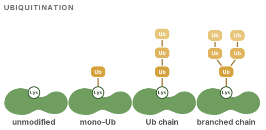
A canonical example of a PTM is ubiquitin. Ubiquitin is itself a small protein domain that's covalently attached to (and sometimes removed from) other proteins. Typically, when multiple copies of ubiquitin are attached in a particular manner, the proteasome[[10]] will destroy and recycle the labeled protein[[11]].
PTMs
Ubiquitination is the covalent attachment of copies of ubiquitin to another protein.
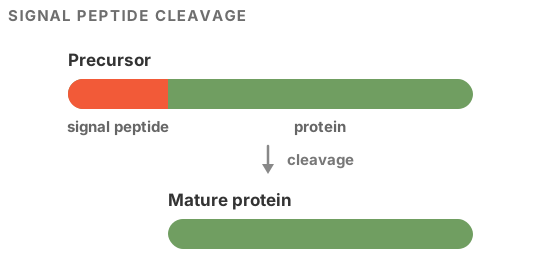
Cleavage, or proteolysis, does the opposite: it removes part of a protein through the action of another (or the same (!)) protein. For instance, many proteins are produced with an attached signal peptide that is usually removed.
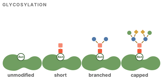
Glycosylation attaches sugar chains, often branched, to proteins. The precise pattern of sugars can change which molecules a protein binds and how the immune system recognizes it. It matters for drugs, too: the antibody obinutuzumab is made with less of the sugar fucose so that it binds more strongly to a receptor on immune cells[[12]].
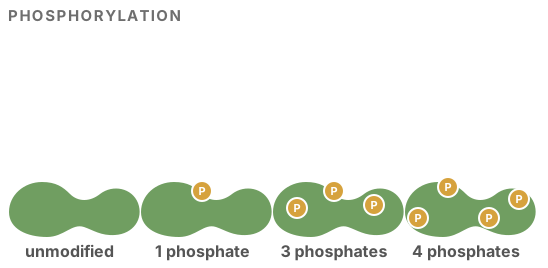
Large classes of PTMs are small modifications to individual amino acids, for instance phosphorylation by kinases. Phosphorylation is used to dynamically regulate the structural ensemble of a protein and change which proteins it will interact with[[13]].
Matching combinatorial complexity with combinatorial measurement
Proteoforms are assembled from a shared vocabulary of component pieces. One obvious consequence of this is that the number of potential—and actually observed—proteoforms is vast[[14]]. We won't bother with the traditional comparison to the number of atoms in the universe, but it's very large.
An example of combinatorial assembly with a few simple components. AMPK contains one α, one β, and one γ chain. The human paralogs allow 12 possible chain combinations. All three chains have been reported as ubiquitinated; α and γ have also been reported as O-GlcNAcylated.
A common tactic in biology is to match combinatorial complexity with combinatorial measurement. The olfactory system is the canonical example, and the same idea has been used in designed measurement systems like MERFISH[[15]]. That's exactly what we propose here. If you read our last post describing our assay, you can probably see where we're going, but let's quickly recap how it works.
In short, Imprint turns transient target–binder interactions into a DNA copying and extension event. When a binder molecule binds to a target, there's a chance an identifying DNA barcode is copied from that binder to the target. The critical property for proteomics is that this happens many times for the same target as binders bind and unbind: we can record about 30 separate binding events in a single short read.
We've already shown that this allows us to measure kinetic parameters for all pairs of interactions between labeled target and binder molecules. But what if we flipped this around and used known binders with known interaction patterns to identify unknown targets?
Imagine you have a collection of unidentified proteoforms floating around in solution. You first attach a non-identifying DNA stub to each of them[[16]]. You then add a carefully designed collection of a few hundred to a few thousand protein binders, each of which has a uniquely identifying DNA tag. Then, you run our assay. As the assay runs, DNA tags from the binders are copied onto the DNA records attached to the target proteoforms. At the end of the run, the records are cleaved and a uniform[[17]] random subset is sequenced.
Each resulting short read contains about 30 recorded binding events involving an individual proteoform and a subset of the binders: with a properly designed set of binders this is a huge amount of information about each proteoform.
As an example, consider a small, stylized family of PD-L1-related proteoforms that differ in two respects: whether PD-L1 is ubiquitinated and whether it is bound to another protein, CMTM6[[18]].
PD-L1 is a cell-surface ligand for PD-1, an inhibitory receptor expressed by T cells. When PD-L1 engages PD-1, it dampens T-cell signaling and can reduce a cytotoxic T cell's ability to kill the cell displaying PD-L1. Tumor cells can exploit this pathway by maintaining high levels of PD-L1 on their surfaces[[19]].
Cells regulate surface PD-L1 partly through ubiquitination, which can direct PD-L1 toward internalization and degradation. CMTM6 associates with PD-L1 and reduces the probability that it is ubiquitinated[[20]], protecting it from lysosome-mediated degradation and thereby stabilizing PD-L1 at the cell surface[[21]].
These distinctions matter for drug development. Several strategies aim to lower PD-L1 by destabilizing it (disrupting CMTM6, promoting ubiquitination, or degrading it directly) rather than blocking it. A drop in total PD-L1 tells you whether such a drug worked, but not how. Does the candidate pull PD-L1 away from CMTM6? Does the ubiquitinated fraction rise? Each of those is a shift between the proteoforms below.
With the biological story out of the way[[22]], we can focus on the problem at hand. We need to distinguish between at least five classes of proteoforms: PD-L1 in isolation, CMTM6 in isolation, PD-L1 in complex with CMTM6, ubiquitinated PD-L1, and ubiquitinated PD-L1 in complex with CMTM6. With our assay we could do this with just three easy-to-design binders: one to PD-L1, one to CMTM6, and one to ubiquitin.
Imagine how hard this would be if we only observed one binding event per target molecule (as in standard affinity proteomics): we'd need specific binders for each of these proteoforms, which would be almost impossible to design.
Each of the five considered proteoforms has a distinct binder signature and can be readily identified from binding events.Multiple component-specific binders interacting with ubiquitinated PD-L1 in complex with CMTM6.
Binding sites
We've transitioned from talking about components of proteoforms to binding sites. These are not the same! For instance, the Ig fold domains in titin and an antibody do not share common binding sites. That's fine—bindable surface features also occur repeatedly across the proteome (for exactly the same reasons).
Technically speaking, we don't really need to measure binding sites at all: we could use highly polyspecific binders that each hit multiple binding sites.
A small-molecule drug-development example: PROTACs
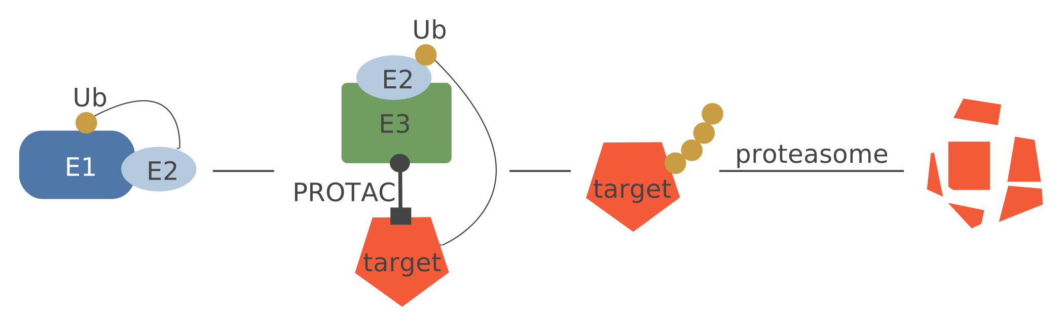
PROTACs bring a target protein together with an E3 ubiquitin ligase, promoting ubiquitination and ultimately destruction of the target. Developing one means debugging a very complex process. Our assay could give detailed mechanistic insight into how a candidate molecule works (or doesn't). Does it induce a complex between the target and E3 ligase? Is the target then ubiquitinated? Does that ultimately reduce levels of the target? How do these responses differ across related proteins?
Distinguishing between five proteoforms with three binders is an impressive trick, but this approach also scales to much larger numbers of proteoforms.
How well would this scale and how much noise could we tolerate?
Math
This section is optional. The intuition behind our approach is simple: we're essentially playing the game of Guess Who with epitopes instead of mustaches and hats[[23]]. Napkin math does give us some insight into how this might work, though:
observing multiple binding events per target is exponentially better than observing one, and allows for high accuracy and coverage.
we should be able to very accurately estimate proteoform abundance (even for rare proteoforms) using DNA sequencing.
binders that hit many proteoforms (e.g., via a shared component) are better for our application than proteoform-specific binders: fewer binders means lower cost and less total off-target noise.
Before we develop a toy mathematical model for our system, we need to distinguish between two closely related tasks that are both commonly referred to as proteomics:
accurately identifying an individual proteoform target from a single read.
measuring the frequency of proteoforms in a diverse sample (often with high dynamic range[[24]]).
We'll discuss both, but in most applications—for instance, trying to figure out how a biological system is responding to a perturbation—the second is more important: we care less about individual molecules than about the proportion of each proteoform in the sample.
Let's say there are \(B\) types of binders and \(P\) proteoforms we want to distinguish between[[25]]. For simplicity, let's start with a forward model for a single read \(r\) generated by ground truth for proteoform \(p\).
Because the order of events in the record doesn't matter[[26]], the read \(r\) is a vector in \(\mathbb{N}^B\) with each entry the number of occurrences of that binder in the record.
Let \(\lambda \in \mathbb{R}_{\geq 0}^{P \times B}\) be a matrix of effective recording rates: \(\lambda_{pb}\) is the rate of recorded events from binder \(b\) on proteoform \(p\), incorporating binder concentration, interaction kinetics, and recording efficiency[[27]]. A reasonable measurement model for \(r\) is
$$ r \mid p \sim \mathop{\text{Multinomial}}\nolimits\left(30, \frac{\lambda_{p\cdot}}{\sum_b \lambda_{pb}}\right). $$
In English: given the target proteoform was \(p\), each binder in the record is an independent sample with probability proportional to its recording rate[[28]]. Dividing the row \(\lambda_{p\cdot}\) by its sum gives the distribution of binder identities conditional on a recorded event. While we're here, let's define a prior distribution over targets (exactly the frequencies we'll estimate later), \(\mathcal{P} \in \Delta_P\). For now, let's assume it's uniform[[29]].
To make this concrete, let's go back to our PD-L1 example, with its five proteoforms and three binders. One possible \(\lambda\), in arbitrary rate units, might be
The small entries represent occasional off-target events. In this illustrative example, we assume that each binding site's recording rates stay the same when it is part of a complex or another site is added. Adding CMTM6 or ubiquitin therefore adds recording opportunities and increases the total rate.
With this likelihood model we can use Bayes' rule to compute a posterior distribution over which proteoform generated each read. Under the assumed model we can then calculate the expected classification accuracy.
Single-molecule classification is impressive, but often we care more about estimating the frequency of each proteoform in the sample—in other words, estimating \(\mathcal{P}\). The model here is also very simple:
Each read is generated by an unknown proteoform \(p_i\), which then emits the observed binder counts \(r_i\).
We can see how the difficulty of estimating \(\mathcal{P}\) changes with the dynamic range in the interactive visualization below. In short, estimating \(\mathcal{P}\) is much easier than classifying individual molecules, and we can theoretically handle a high dynamic range by sequencing deeply.
You can come up with different \(\lambda\)s to simulate a particular proteoform family of interest to you. A critical modeling assumption is the structure in \(\lambda\): basically, which subparts make up your proteoforms, how binders interact with them, and how they're distributed. For instance, in the PD-L1/CMTM6 example above, with the binders we chose we'd be unable to distinguish between ubiquitin attached to PD-L1 and ubiquitin attached to CMTM6. For some applications this wouldn't matter. But if it did, you could add binders to the interface (much easier than it sounds, because they don't have to be perfectly specific!).
As a more realistic example, let's consider a family of proteoforms at the center of a lot of current drug development: Cullin–RING ligases (CRLs). CRLs are modular complexes that attach ubiquitin to other proteins, usually marking them for destruction. Each is assembled from interchangeable parts: a cullin scaffold (here CUL4A or CUL4B, each carrying its partner RBX1), the adaptor DDB1, and one of dozens of substrate receptors that decides which proteins get tagged.
Shown are the ten forms of one receptor, CRBN, which is recruited by many PROTACs: on its own or built into a ligase, with or without the small protein NEDD8 that switches the ligase on, and with or without ubiquitin on CRBN itself. Any of nine other receptors can take CRBN's place, giving a total of 105 proteoforms. Amazingly, they can in theory be identified with just 17 binders; in simulation, a single read identifies its form 99.3% of the time.
Measuring 105 CRL4 proteoforms with 17 binders
Maximum-likelihood estimates of all 105 CRL4 proteoforms from simulated reads, with illustrative abundances spanning seven orders of magnitude and about 15% of binding events off-target. The common forms are measured accurately with about a million reads; the rarest, roughly one in ten million, appear only after tens of millions.
The same holds at larger scale: in a simpler simulation with 1,000 protein chains and two specific binders for each, abundance estimates also converge with read depth across many orders of magnitude.
All of this assumes we know the recording rates \(\lambda\) exactly. In practice we won't: binder concentrations and activities drift. In the next simulation we add multiplicative error to each binder's rate; we can then jointly estimate proteoform frequencies and the multiplicative factors.
Fitting with misspecified binder rates
Reads are simulated with each binder's recording rate multiplied by the factor shown on the right. Despite this, jointly estimating the multiplicative error and the abundances gives nearly the same accuracy as when the rates are known exactly.
One nice aspect of a sequencing readout is that you can get a relatively large dynamic range just by sequencing deeply, but there are other games one can play. For instance, for samples where we have some idea of the distribution, we could adjust the concentration of different binders to compensate, or introduce bias into the initial DNA stub attachment process.
Why this approach to proteomics?
Protein sequencing is an amazing emerging technology with many applications, but proteoforms, unlike DNA, are fundamentally not linear stores of information. If you can only sequence a single chain, you lose critical information about complexes and many PTMs.
Existing affinity proteomics platforms like Olink[[30]] and SomaScan[[31]] already read out binding with DNA, but they rely on one highly specific reagent (or matched antibody pair) per target, limiting coverage and accuracy. The closest idea to ours is Nautilus's multi-affinity approach[[32]], which also identifies single protein molecules from the binding patterns of many moderately specific probes. We'd do this in a single pooled reaction (with many, many binders) rather than over rounds of imaging and washing[[33]], read out with DNA sequencing, and work with native complexes in solution.
Mass spec enables a plethora of beautiful, high-accuracy approaches to proteomics, but so far has not become nearly as widespread as DNA sequencing-based technologies like RNA-seq.
Altogether, we'd have high resolution and coverage of proteoforms, low cost, and high accuracy. We'd also have much less stringent binder design and verification needs compared to traditional affinity approaches.
Could we pull this off?
Hopefully we've convinced you that this idea could work, at least in theory. Getting from this sketch to a viable implementation will require some further development.
On the binder design side, we think this would be difficult, but not impossible. Unlike most affinity tech we don't need high-affinity or high-specificity binders—in fact, moderate-affinity minibinders are ideal. We're not bad at designing these things. We'd also have the advantage of an absolutely bonkers method for testing many binders against huge panels of targets[[34]].
For PTMs, nature has already solved a version of this problem. Cells read modifications with moderate-affinity, polyspecific domains: SH2 domains recognize phosphotyrosine plus a few flanking residues, 14-3-3 proteins and FHA domains read phosphoserine/threonine motifs, lectins read glycans, and ubiquitin-binding domains like TAB2's NZF or NEMO's UBAN distinguish chain linkages. Each recognizes a modification in a local context rather than one site on one protein—exactly the kind of binder we want. Most are too weak for wash-based affinity assays, but Imprint records transient interactions, so weak binding isn't a problem.
We'd need to further develop Imprint for this application to maximize the number of informative extensions per read, reduce background noise, and handle complex biological samples[[35]], but we've already shown the underlying technology measures the relevant biophysics. We've focused on measuring complexes, which might require modeling spatial effects, though of course there are many applications where measuring large complexes is not required.
The payoff for pulling this off is hard to overstate: we'd be able to generate data about biological systems at unprecedented scale and resolution[[36]].
[[1]]: Friedrich Engels, "Notes and Fragments," in Dialectics of Nature (written 1870s–1882; first published 1925). See Philip Ball, How Life Works (2023).
[[2]]: We'll use fold and domain roughly interchangeably. For a visual overview of domains in the AlphaFold Database (AFDB), see TED.
[[3]]: Tandem domain repeats such as titin's are especially common in eukaryotes and often expand through internal duplication of several domains at once. Åsa K. Björklund, Diana Ekman, and Arne Elofsson, "Expansion of Protein Domain Repeats," PLoS Computational Biology 2, no. 8 (2006): e114.
[[10]]: Which is itself a complex and variable modular assembly of subparts subject to modifications.
[[11]]: Though of course not always; ubiquitin has a diverse set of uses. Also, as always in biology, there are many subtle variations on this theme, such as the ubiquitin-like proteins NEDD8, SUMO, and so on.
[[22]]: By the way, developing this story required many individual assays and experiments; ideally one could measure all of these properties at once.
[[23]]: Okay, really we're playing the classic variant of Guess Who where we ask hundreds of questions at once and receive a subsampling of the questions for which the answer is "yes" in return.
[[24]]: A wide gap between the most frequent and least frequent interesting proteoforms. In biological systems this can be many orders of magnitude.
[[25]]: Really, we're always going to be talking about equivalence classes of proteoforms. That's fine.
[[26]]: After some clever tricks to avoid repeated extensions from strong binders (the very feature we exploited in our last post). Also, order really does matter and we can exploit it, but this is a simplified model.
[[27]]: You could derive these effective recording rates from a kinetic model and binder concentrations, but in practice it's probably better to fit them empirically, up to the row scales that this fixed-length read model can't identify.
[[28]]: This assumes we're maxing out the short read. Otherwise we'd replace this with a truncated Poisson, which is also easy to simulate.
[[29]]: For this thought experiment we'll use a uniform prior. In practice, however, this is absurd: proteomics samples often exhibit extreme dynamic range and we'd often have a reasonable way of knowing something about which proteoforms are present (e.g., by RNA-seq, or by doing some selective pulldown).
[[33]]: Compared to wash-and-image combinatorial approaches we'd be less limited by the number of rounds—we could use thousands of distinct binders rather than a few hundred. We'd also avoid sequential washing and denaturing: Nautilus binds "intact, denatured protein molecules" to its flow cells.
[[34]]: There are, of course, difficult epitopes in the proteome. Also, for more exotic PTMs and applications where you'd want spatial resolution, binder design might be a bit harder. Again, better data and models will help.
[[35]]: For instance, membrane and DNA-binding proteins are currently impossible. Our initial PD-L1/CMTM6 example would be quite difficult for us to handle currently.
[[36]]: We'll get more into the motivation for developing this technology in a future post. But in short: we think the real value of AI in biology is in predicting how biological systems will respond to interventions.