How to sequence fundamental biophysics

Akshay Tambe, Daphne Chen, Mohamed Ghazal, Nick Boyd - 08 Sep, 2026

We can quantify the kinetics of a million protein–protein interactions in one tube by generating and sequencing time-resolved DNA records of binding events.

Last time, we walked through what it would take to build a protein model that really understands biophysics. We talked about the nature and scale of the data it would take to get there and we vagueposted about the assay we’ve developed to generate it. We told you that we did a sequencing experiment and somehow measured multiple protein–protein interaction rates with remarkable accuracy and precision.

In this post, we explain our assay at a high level. We describe how we built this new workflow from the ground up: from a theoretical foundation to a method for getting multiplexed kinetics and binding data from a single tube measured at a single time point.

We won't go deep into why we built it this way in this post. But suffice to say that when we started the company, we wanted to take a step back and ask: what would it look like to design this assay for the ML age? That required rethinking how protein interactions are measured from scratch — moving beyond individual wells and small batches to a system that scales massively.

Reductions: A handy way to simplify problems

Measure a biological process with DNA sequencing and scalability goes through the roof

We’ve found that leaning on concepts from computer science is a really helpful way to reframe biotechnology development around fundamental requirements — in this case, scalability.

In computer science, a reduction is a tool to convert one problem into an instance of another problem that’s already been solved. Originally, reductions were purely theoretical, but nowadays they’ve become a key tool that let computer scientists solve real problems. Imagine a computer scientist at Lyft is given a new task, like “which nearby driver should get matched to this rider?” They might ask: does this problem reduce to one of a handful of canonical problems we can solve efficiently? Perhaps they’d land on “shortest paths,” using it to estimate each driver's pickup time by treating roads as a map of distances — then matching the rider to the driver who's closest.

This phenomenon is at work in modern biology even if it isn’t recognized as such: many scalable measurements are reductions to DNA sequencing. There’s good reason for this: DNA sequencing has become absurdly good by almost any metric you choose. For a few thousand dollars, you can generate tens of millions of high-quality DNA sequence reads in a sequencing run that takes only a few hours.[[1]]

The implications of this are profound. If you can come up with a clever way to reduce your measurement problem to DNA sequencing, you not only don’t have to develop entirely new instruments and tools — you automatically get immense scale for free. The trick is to find the right molecular ingredients to carry out the reduction.

Scooby-Doo unmasking meme: “cool new technique” is pulled off to reveal “DNA seq” underneath.

Below are some example biological measurements that have been reduced to DNA sequencing, with notes on the key molecular ingredients that make each one work. As you go down the list, you’ll notice they sound less and less related to DNA itself. This is the beauty of reducing a measurement to DNA sequencing — the process you’re studying doesn’t need to have anything to do with DNA.

RNA abundance: To quantify RNA on a DNA sequencer, use a reverse transcriptase enzyme.[[2]]
RNA secondary structure: To detect the basic shapes RNA can fold into, use a simple chemical tool that deposits an adduct in a structure-dependent manner, and a polymerase that records these adducts as a mutation.[[3]]
Accessibility of the genome: To discover which portions of the genome are actually being used in a particular cell, use a hyperactive transposase, like in ATAC-seq.[[4]]
Drug-like molecules: To screen drug candidates (when you’re a genomics scientist who doesn’t want to learn chemistry), use DNA-encoded libraries (DELs).[[5]]
3D locations of molecules in a cell: To map out where molecules are in a cell, use DNA microscopy.[[6]]
Dark matter?: Sounds crazy, but there are some really serious proposals about using sequencers to detect dark matter.[[7]]

You can probably see where we’re going with this. One of the core problems we’re working on at Escalante is how can we use a DNA sequencer to quantify protein interactions at scale.

What we want is gold-standard biophysical data: the actual kinetics parameters for all interactions, at a massive scale and with $O(1)$ experimental complexity (another concept we’ve borrowed from CS to better think about scalability). The current options just don’t cut it — the data quality from SPR and BLI[[8]] is great, but their $O(n^2)$ experimental complexity limits throughput. Phage display has better $O(n)$ experimental complexity, but it yields low-quality data and it provides only relative enrichment values rather than absolute, quantitative measurements.[[9]]

We knew we’d have to build something totally new, and the rest of this post is dedicated to explaining what it looks like.

But first, if biochemistry and biophysics are newer to you, the “Biochem 101” section below covers core background to help you understand our assay and the data it provides.

If you’re already steeped in molecular bio, skip straight to “Molecular implementation” (or open the toggle to get a refresher and play with the binding kinetics simulator)!

Biochem 101

We can describe the way proteins interact with a handful of key terms and measurable biophysical values

At the molecular level, interactions between proteins aren’t static[[10]]. Molecules move and change over time. Imagine a single molecule, we'll call it the “target,” floating in a solution of molecules that can grab on or “bind” to it, which we call, unsurprisingly, “binders.” Over time the target gets hit by binder molecules bouncing around. Sometimes this does nothing and the binder just bounces away (perhaps the wrong face of the binder collided with the target or they don’t interact). But sometimes such a collision results in a binding event, where the binder and target stick together in a “complex.” The average time it takes for a binder to bind its target is captured by a term called the “unbound half-life.” This is an innate property of the biophysics of the target and binder, and directly influenced by the concentration of the binder (if you double the concentration of binders, you double the number of collisions).

Similarly, a binder–target complex doesn’t persist forever. These complexes are jiggling around and jostling into other stuff, and eventually the binder falls off (which we call unbinding or dissociation) and the molecules diffuse away from each other. The time they stay bound is parameterized by the “bound half-life,” another key biophysical property of the binder–target complex.

Biologists typically use the reciprocal of these half-lives, which are called kinetic rates. $k_{\text{off}}$ (measured in $s^{-1}$) is the inverse to the half-life of the bound state, and $k_{\text{on}}$ ($s^{-1}\,M^{-1}$), which is related to the half-life of the unbound state. And in some cases, these two rates are summarized into a single parameter, $K_{\text{D}} = \frac{k_{\text{off}}}{k_{\text{on}}}$ (Figure 1). This is lossy, and there are infinite $k_{\text{off}}$ and $k_{\text{on}}$ that give rise to any given $K_{\text{D}}$ value, but it does have its uses, and in some cases, it’s easier to measure directly than $k_{\text{off}}$ or $k_{\text{on}}$.

Fig. 1: Adjust $k_{\text{off}}$ and $k_{\text{on}}$ to see how they impact $K_{\text{D}}$.

Molecular implementation

We infer the duration of binding interactions from reads generated by isothermal proximity extension

In our assay, we’re trying to measure which pairs of proteins interact with each other, and for how long. There’s both a spatial component — interacting proteins are close together — and a temporal one — interacting proteins stay in proximity with some half-life. We can measure each of these components in a unique way. We ultimately do this by combining proximity extension with isothermal amplification.

That's a mouthful, so let's build it up one piece at a time.

Proximity extension to capture spatial information

DNA is only amplified when proteins are close enough to interact

We'll start with proximity extension assays. These are well-established and, unlike the temporal part of our assay described in the next section, we didn’t need to do much tweaking to apply this strategy for our purposes.

So what is proximity extension? As the name suggests, it’s a way to selectively extend DNA only when two molecules are physically close to each other. Before we get into exactly how it works, you need to understand that it relies on a variation of classic PCR called overlap extension assembly. In this strategy, you have two templates that share a bit of matching sequence. When the templates encounter each other, they “base-pair” into an overlapping form that lets a DNA writing enzyme (polymerase) extend them, copying information from one template onto the other (Figure 2). The polymerase can’t act on the original templates before they base-pair because it can only copy from a single strand, and the templates start double-stranded.

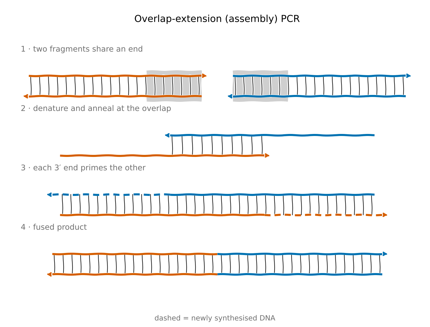
Overlap-extension (assembly) PCR in four steps: two fragments share an end; denature and anneal at the overlap; each 3′ end primes the other; fused product. Dashed strands are newly synthesised DNA. — Fig. 2: Overlap-extension (assembly) PCR joins two DNA fragments that share a complementary terminal sequence. (1) The two fragments carry an overlapping end. (2) After denaturation, the complementary ends anneal to one another. (3) Each 3′ end then primes synthesis across the other fragment, extending both strands. (4) The result is a single fused product combining both fragments. Dashed lines denote newly synthesized DNA. Our assay uses a similar concept for barcoding.

From a data vantage, information that was originally on two separate strands ends up on a single strand. This is a really useful molecular operation — many reductions to DNA sequencing work by tracking how DNA sequences are copied and rearranged according to these very well-understood rules.

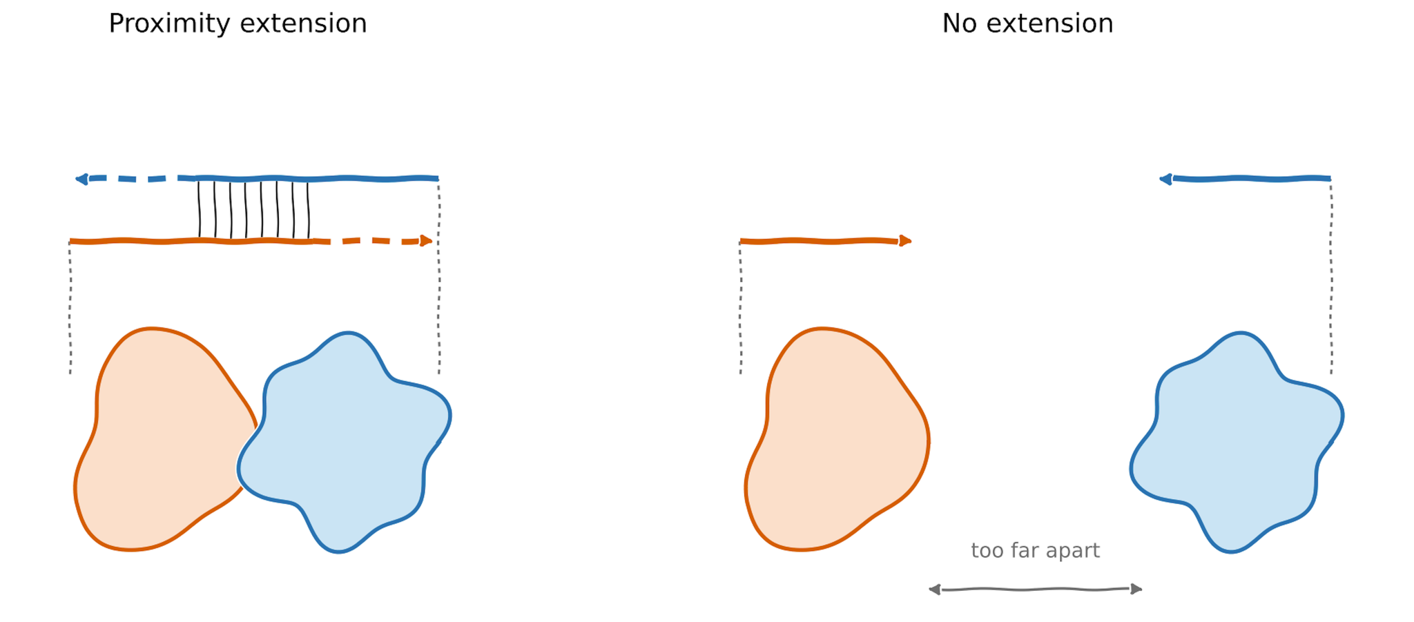
Now for the “proximity” part (Figure 3). The setup involves two proteins, each with its own barcoded DNA tag (a barcode is a unique DNA sequence that we can add to help track where a piece of DNA came from even when it’s mixed among thousands of others). When these tagged proteins are just floating around in solution nothing happens; the DNA strands are too far from each other for a productive copying event. But if they both bind to each other, this anchors them in space near enough to each other, allowing the two strands to pair and serve as the template for overlap extension. So if we see extended DNA with the unique barcodes from those two proteins (these will be among the “reads” output from the sequencing experiment), it means those proteins interacted.

If you’re trying to measure protein–protein interactions in detail (and not, say at the scale of a whole cell), this is a really tidy simplification. The vast majority of DNA tags don’t generate data since when the protein carrying them isn’t bound to a target, they’re not close to the target’s matching strand, and overlap extension can’t happen[[11]].

Proximity extension: two proteins bound together hold their orange and blue DNA tags close enough to base-pair, and each strand extends past the overlap. No extension: the same two proteins sit too far apart and their tags never pair. — Fig. 3: Principle of proximity extension. Left: when two proteins are near each other, their complementary DNA tags pair together, allowing a polymerase to extend the DNA to create a detectable amplicon (proximity extension). Right: if the proteins are not bound, the DNA tags cannot pair and thus no extension occurs.

Isothermal amplification to capture temporal information

Barcodes are copied at a known rate, so we can use the number of copies to determine duration of a protein–protein interaction

Proximity extension is a great starting point for the spatial side of our problem, but encoding temporal information is less straightforward. While designing this, we considered doing the inelegant thing — manually collecting a bunch of time-points — and weren’t convinced. We’re building these workflows as data generators for ML, and want data on time-scales that may be too fast for manual pipetting, and with reproducibility and resolution that manual (or even automated) pipetting can’t cope with.

We turned to DNA microscopy for inspiration. Without getting into detail, this is a technique that generates a model of molecule positions in a cell without any actual microscopy[[6]]. Instead, it relies on the fact that pairs of DNA-tagged molecules that are closer together in distance are more likely to find each other, letting their tags base-pair and unique barcodes get amplified. Thus, when you look at read counts in aggregate, more reads of a given barcode pair means those molecules originated closer together, whereas fewer reads means they’re farther apart. Throw in some math and you can generate a whole map of molecules across a cell.

We reasoned that we might similarly design a scheme wherein a read containing any single barcode pair means little, but looking at read counts in aggregate might tell us temporal information. We figured that for any temporal data to be high resolution, we’d need a process that can write more than the one barcode that proximity extension gives you.

Unfortunately, standard overlap extension doesn’t cut it. Like in standard PCR, after polymerase copying, you end up with double-stranded DNA that needs to be melted apart with heat before you can continue the process. But alas, high temps would also unfold the proteins we’re trying to study.

We turned to isothermal linear amplification. This approach relies on a family of DNA writing processes[[12]] that work at a single temperature (aka isothermally), so we don’t have to repeatedly heat things up and ruin protein structure. And, crucially, the polymerase writes barcodes at a known rate that is biophysically fixed — in other words, a molecular clock.

That’s it! At the molecular level, our spatiotemporal protein interaction sensor works by hooking proximity extension onto isothermal amplification.

Putting it all together

Our assay turns binding event measurements into a DNA sequencing readout

The key concept
The longer a pair of proteins are bound together, the more time DNA polymerase has to write barcodes, and the more barcodes we ultimately see. This means we can use the number of barcodes as a proxy for the amount of time the proteins spent together.

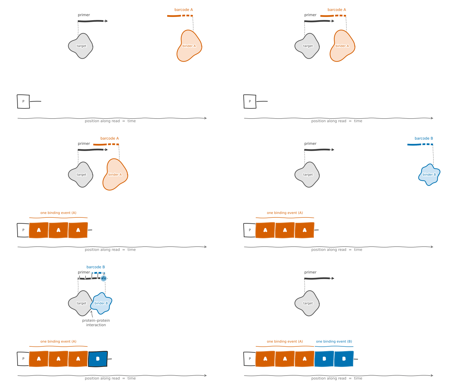
Animation of proximity barcoding. A target carrying a primer and binders carrying barcodes dock and release while a polymerase extends one strand; an axis below reads “position along read = time”. — Fig. 4: Proximity barcoding. When a binder engages the target, the polymerase copies the binder's barcode onto a single growing strand, repeating it for the lifetime of the complex (orange "A" run); the next binder appends its own barcode (blue "B" run). Read position encodes time, so the sequence records which pairs interacted and for how long. For simplicity, we don’t show the large polymerase molecule that “writes” new DNA.

Here’s how it works in more detail (Figure 4). One of the proteins — the binder — has a piece of DNA attached to it encoding a barcode that can be copied onto a new strand. The other protein — the target — has DNA attached to it that can be extended as new barcodes are written onto it. When these molecules are not interacting, nothing happens (much like proximity-extension assays). But when they bind to each other, the DNA strands they carry are able to pair up, and the polymerase can get to work writing new DNA.

The polymerase starts copying barcodes into the strand it extends. Critically, these barcodes don’t fall away as a bunch of separate molecules — instead, they’re connected into a single growing strand (orange As in Figure 4). A long-lived interaction produces a contiguous run, repeating that binder's barcode until the complex falls apart. Whatever binds next starts a new round of barcode copying (blue Bs in Figure 4). Once we sequence this stretch of DNA, we can essentially read how long different pairs of proteins were bound together over time.

This makes the reads incredibly rich: they tell you which binder and which target interacted, and for how long.

Data: What comes out of a real experiment?

Our assay generates clean reads from which we can extract key biophysical metrics

We’ve shown you how the assay works conceptually. Next, we’ll share what outputs look like and what kinetic properties we can pull out mathematically.

Check out some actual reads

We’ll skip the engineering and debugging that it took to implement all this in the lab and jump right to the reads. Each read contains the following fields:

A target prefix that tells you, say, “this read came from target 1”
A list of binder barcodes that consist of:
1. A barcode that specifies which binder you’re looking at (perhaps binder design 1, design 2, and so on)
2. A unique molecular identifier (a UMI[[13]]) that helps distinguish between two otherwise equivalent molecules of binder design 1 (this helps us count reads correctly)
Various boilerplate fields to make the molecular biology work

Here are some actual reads. This is the raw stuff straight off the sequencer: no error correcting, no human twiddling, no nothing.

Interactive read viewer — step through individual sequencer reads and their decoded barcode segments.

Turning sequencing reads into binding kinetics data

So each read is a series of binding events in (discretized) time, where the binders are uniquely identifiable and information about the unbound state is hidden. What kinetic properties can we extract from reads like this? We won’t really get into the math, but here’s the gist:

$k_{\text{off}}$ is the simplest — it’s clear from our reads how long two molecules were bound together before they dissociated. By pooling all of these “dwell times” for a given binder–target pair and fitting the distribution, we can pull $k_{\text{off}}$ out as the decay rate.

$K_{\text{D}}$ is a murkier signal, but we’re convinced our data contains signal here as well. The amount of time a target spends bound by a binder is proportional to the number of barcode events that binder–target pair generated. In other words — this is the bound fraction, a term that gets you halfway to $K_{\text{D}}$. And while we cannot directly observe the unbound fraction (the other term you need to calculate $K_{\text{D}}$), our assay is inherently a competition experiment where many binders vie for the same limited set of target binding sites. The math gets a bit complicated here, so we’ll leave it at this: we think our data contains relative $K_{\text{D}}$ for all binder–target pairs, but that signal is a bit harder to tease out.

Once we have $k_{\text{off}}$ and $K_{\text{D}}$, we can estimate $k_{\text{on}}$, since $K_{\text{D}} = \frac{k_{\text{off}}}{k_{\text{on}}}$.

With these rates in hand, we’ve quantified the fundamental biophysical interaction between a given pair of proteins. And in our one-tube assay, we estimate that we can generate this data for something on the order of a million protein pairs.

How well is it working?

We were satisfied to see that whatever we were measuring was extremely reproducible (Figure 5A). Next, this experiment contained a bunch of binders with interaction kinetics that were independently measured with BLI. Comparing this ground-truth BLI signal to our data (Figure 5B) showed excellent agreement; we can measure $k_{\text{off}}$ about as well as the gold-standard process does over a useful working range. As we alluded to before, $K_{\text{D}}$ is trickier to find. We have some ideas for how to tease it out from our data and are running experiments. More to come soon.

Precision: estimated k_off in technical replicate 2 against replicate 1, points on the diagonal, Pearson r = 0.999 and median fold difference 1.04×. — Fig. 5: **A (Precision)**: estimated $k_{\text{off}}$ over two technical replicates; the dashed line marks identical estimates between replicates (Pearson $r$ = 0.999; median fold difference 1.04×). **B (Accuracy)**: BLI-measured versus estimated $k_{\text{off}}$; the dashed line marks agreement with BLI and the green band spans within 2× of the BLI value. In both panels, filled circles denote interactions detected on target and hollow circles denote dropouts (BLI binding without on-target assay detection).

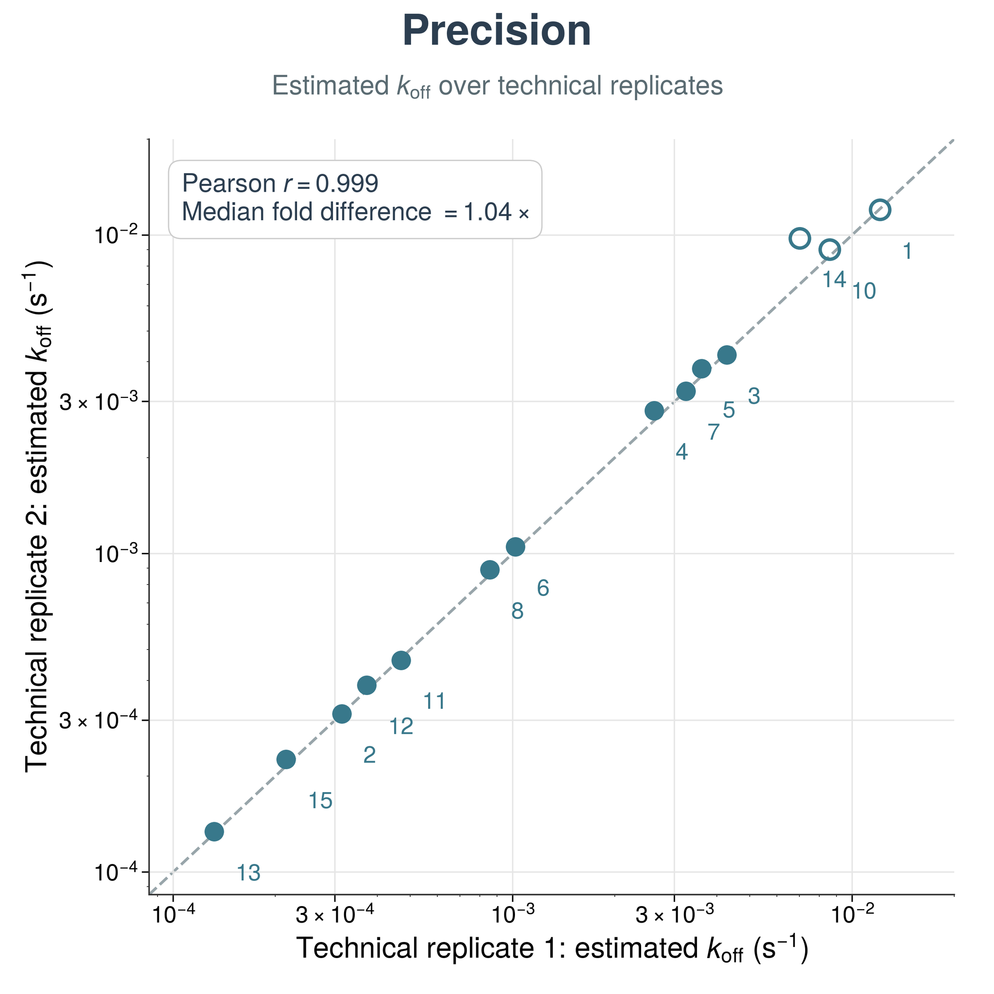
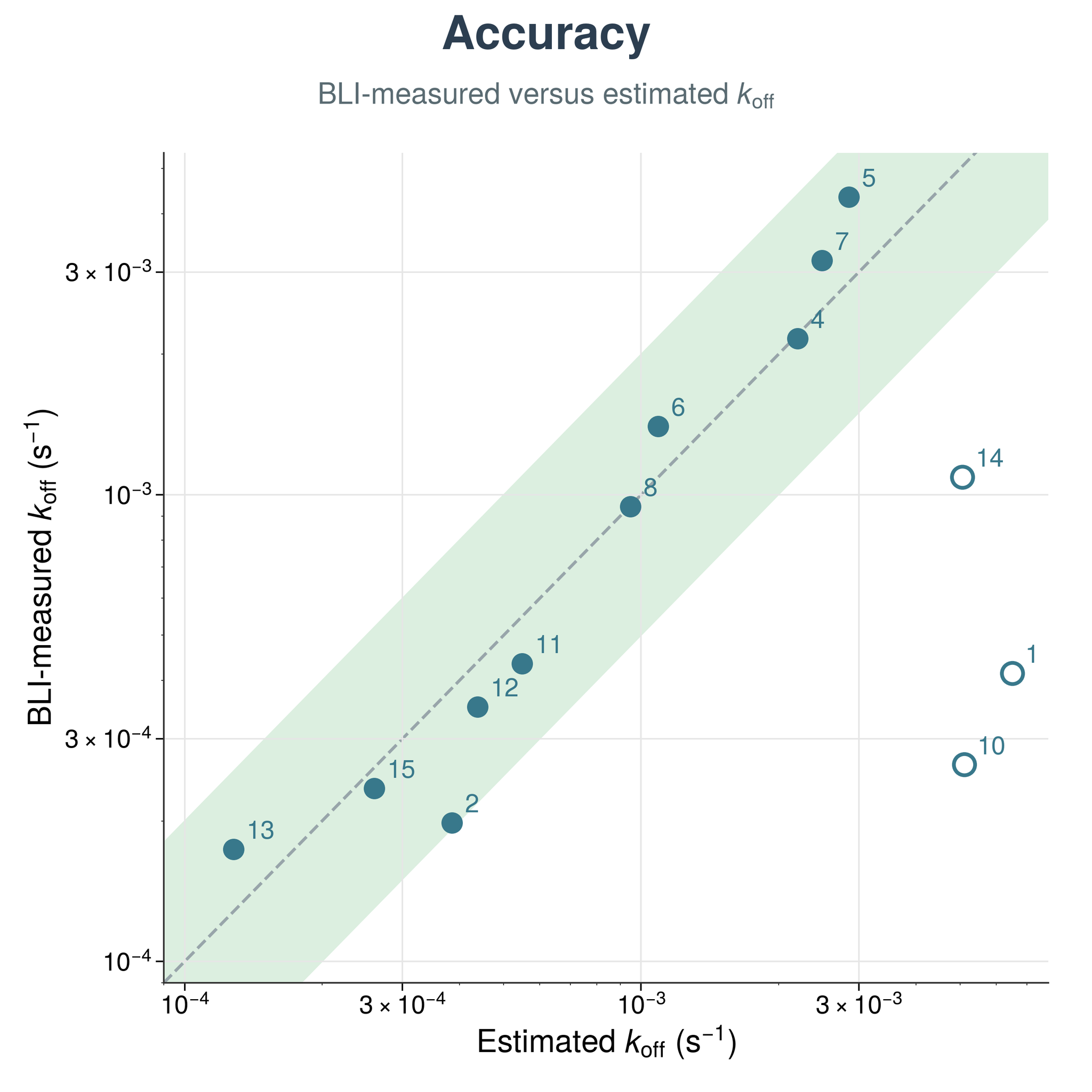
Accuracy: BLI-measured against estimated k_off, most points inside a green band spanning within 2× of the BLI value. Filled circles are on-target detections, hollow circles are dropouts. — Fig. 5: **A (Precision)**: estimated $k_{\text{off}}$ over two technical replicates; the dashed line marks identical estimates between replicates (Pearson $r$ = 0.999; median fold difference 1.04×). **B (Accuracy)**: BLI-measured versus estimated $k_{\text{off}}$; the dashed line marks agreement with BLI and the green band spans within 2× of the BLI value. In both panels, filled circles denote interactions detected on target and hollow circles denote dropouts (BLI binding without on-target assay detection).

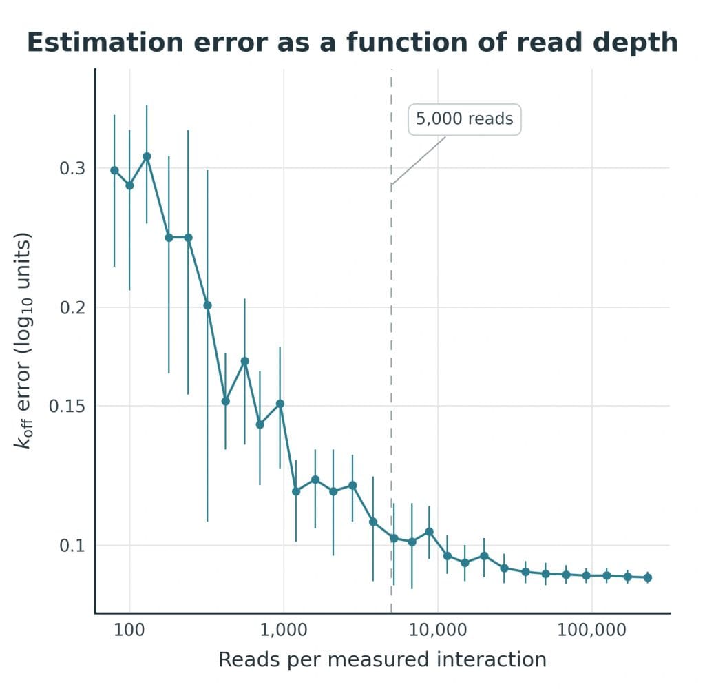
Because of limitations imposed by the sequencing hardware itself, our DNA records are limited to around 25 barcodes per read. This seems like a tremendously coarse way to get temporal info. So how were we able to get such accurate off-rates? The answer is read depth. While the noise floor of our experiment is set by the hardcoded rates of our isothermal extension process, above that threshold, accuracy improves with read depth. For tighter error bars, just sequence more!

Yet we didn’t even need to throw a gargantuan number of reads at the problem. We think we can get accurate estimates with as few as 5,000 reads per interaction (Figure 6); this suggests we can learn about 1 million interactions with a single NovaSeq run. That’s 1 million interaction datapoints for under $10,000 at the current sequencing prices and all done in a one-pot overnight reaction read out in just a few hours on a sequencer.

Estimation error in k_off against reads per measured interaction, on a log x axis. Error falls from about 0.3 log10 units near 100 reads and flattens below 0.1 past a dashed line marked 5,000 reads. — Fig. 6: Calibration error in $k_{\text{off}}$ versus reads per interaction. Error rapidly declines as read depth increases and stabilizes at ~5,000 reads per interaction (dashed line), where the $k_{\text{off}}$ error reaches ~0.1 $\log_{10}$ units.

So where do we go from here?

Focusing on massive scale unlocks massive potential

We’re incredibly excited by this. We really believe this is a new way to measure protein interactions. And it scales ridiculously well; well enough to train models on. To use the terminology we’ve previously expounded, getting to a large interaction matrix usually has wet-lab complexity of $O(n^2)$. We’ve done this in $O(1)$, and things are scaling nicely (Figure 7). And what we measure isn’t just some affinity score that needs its own calibration; it's real kinetic data with solidly grounded biophysics behind it.

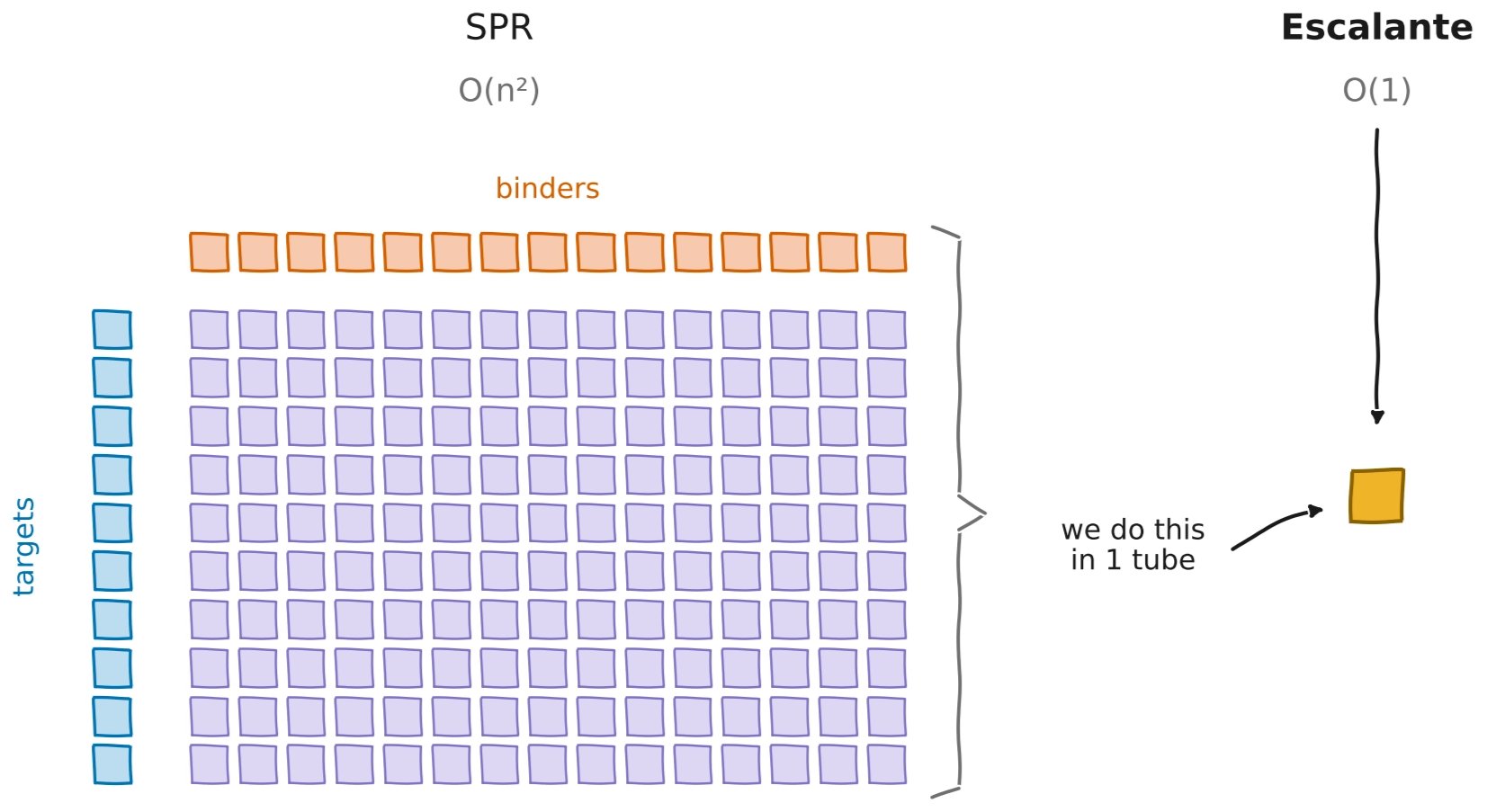
SPR needs an n-by-n grid of binder–target measurements, O(n²). Escalante measures the whole matrix in a single tube, O(1). — Fig. 7: Scaling of interaction measurement: SPR versus Escalante. Pairwise methods like SPR measure one binder–target combination at a time, so a full matrix scales as $O(n^2)$ — a 96 × 96 matrix requires 9,216 separate measurements. Escalante measures all pairs together in a single reaction, reducing wet-lab complexity to $O(1)$.

Imagine that every time you design a binder, you can immediately measure its on- and off-target binding across the proteome just as easily as you measure on-target binding today with SPR or BLI. Collect enough of this data and you could even train a model to predict this. Or imagine if we could design a binder to bind not only a specific protein, but a specific modified proteoform[[14]]. Such single-nucleotide precision is trivial for nucleic acids (via qPCR probes and the like); why can’t we do this with protein-focused assays like Western blots or FACS? Designing specific binding should not be hard. But it is, because it needs to be supported by kinetics data, at massive scale.

We started this post by talking about reductions, and that’s where we’re going to end as well. Beyond our initial assay, what’s really thrilling to us is that applying the reductions in biology has truly transformative potential. Having a cheap, scalable, single-molecule kinetics measurement engine unlocks all sorts of other applications that go way beyond just measuring protein–protein interactions, because many protein-centric problems can be reduced to protein interaction kinetics.

This parallels plenty of other protein sequencing platforms that work by measuring similar interaction kinetics[[15]], but those have less scalable biophysical readouts. And although there may be some other scalable ways to measure protein interactions by DNA sequencing, these depend on living cells, and you can’t build a robust proteomics tech stack on top of a yeast replication cycle.

But you can build it on top of molecular biology and DNA sequencing.

Coming up

In our next posts, we’ll dig deeper into how we came up with this assay at all and how it scales up, how to get the full set of interaction parameters (i.e. not just $k_{\text{off}}$), and we’ll explore applications of this technology beyond protein interactions.

Sign up for emails about new posts at the bottom of this page, and reach out directly if you're interested in working together: hello@escalante.bio.

[[1]]: One place where this manifests is in the cost and scale of sequencing, which you can see in this plot from here.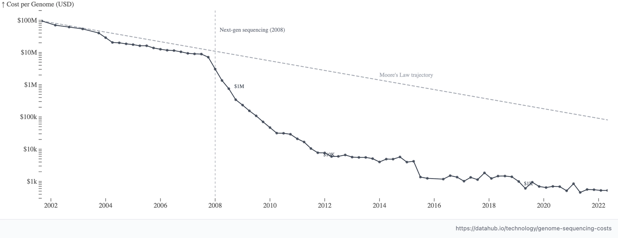

[[2]]: Two of the earliest papers (that we’re aware of) that do this are from these from the Snyder and Wold groups.

[[3]]: As workflows reduce weirder and weirder things to DNA, it becomes common for methods to have equal weight placed on experimental and computational innovation. The original SHAPE-seq work shows this nicely, with a lab-focused paper from Lucks and a companion bioinformatic work from Aviran.

[[4]]: The earliest paper that we’re aware of is this one from Buenrostro. If there's something earlier, please let us know!

[[5]]: DEL workflows combine combinatorial chemical synthesis with DNA writing to output small molecule–DNA conjugates where the DNA tag identifies the small molecules. Then some biochemical assay separates molecules in space (for example, molecules that bind to a protein stay on a solid resin, while unbound molecules are washed away) and a DNA sequencer measures abundances. In other words, DNA-seq ranks molecules by binding strength. DELs were first prophesized by Brenner and Lerner, and Needels implemented in the lab not long afterward. There are also more sophisticated DEL setups where the DNA tag actually contains instructions about how the small molecule was created; these instructions can even be “executed” to generate more copies of the target molecule (this subtlety captures the difference between DNA-recorded and DNA-templated library synthesis, see this perspective.)

[[6]]: This is an absolutely wild work from Weinstein, Regev and Zhang, but perhaps the lay-friendly press release is less daunting. We find this fascinating and plan to write more on this in the future.

[[7]]: See this arXiv preprint from Drukier.

[[8]]: SPR and BLI are workhorse techniques that measure interaction kinetics between a binder and target protein. Both rely on immobilizing one of the binding pair on a surface and (each with their own very complex physics) detect the in-solution binding partner binding onto or unbinding from this surface in real time, with impressive sensitivity. These data are a direct measurement of $k_{\text{on}}$ and $k_{\text{off}}$. For a nice review about how this is done, see this work.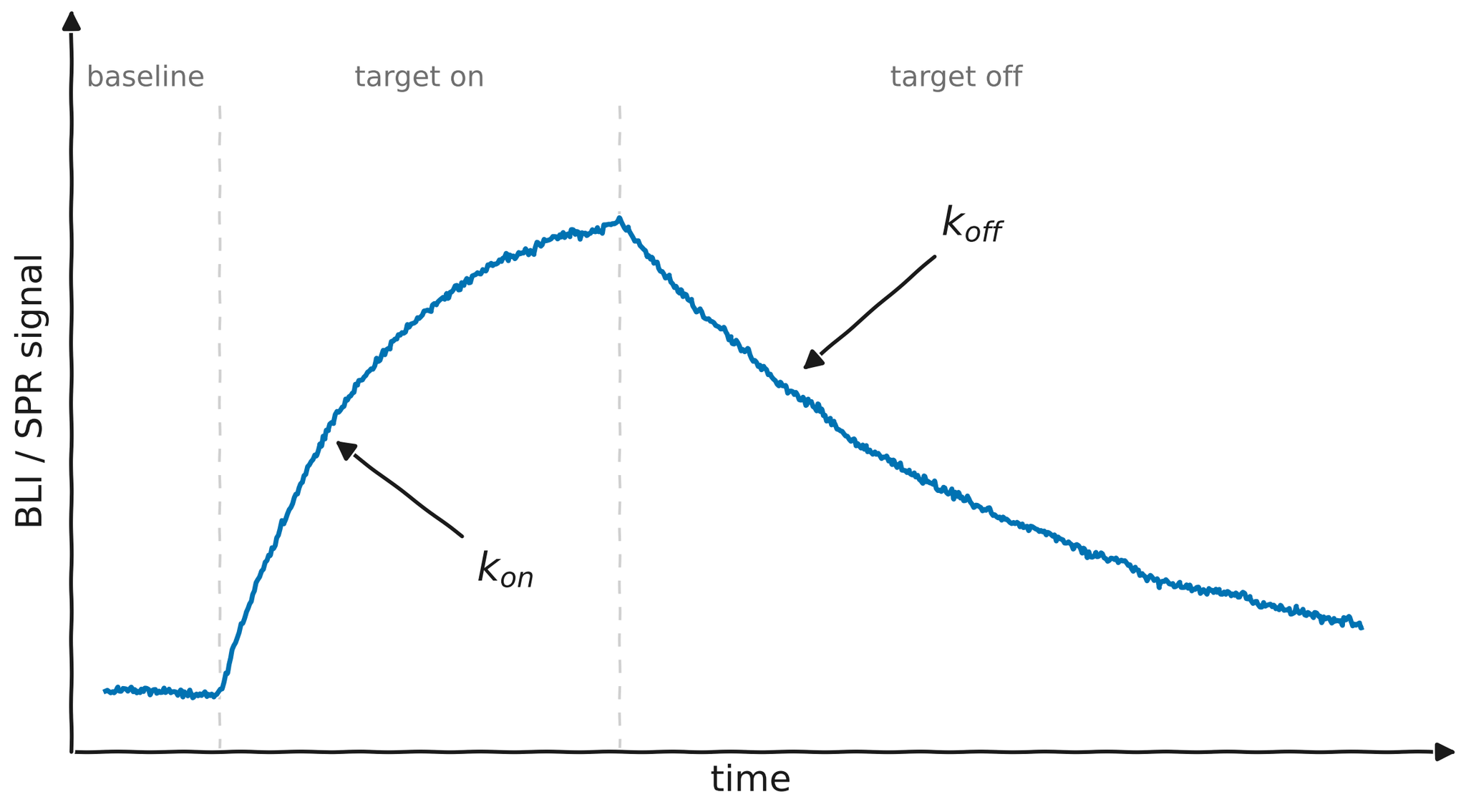An SPR/BLI sensorgram showing baseline, association ($k_{\text{on}}$) upon exposure to analyte, and dissociation ($k_{\text{off}}$) upon return to buffer. Binding affinity is calculated as $K_{\text{D}} = \frac{k_{\text{off}}}{k_{\text{on}}}$.

[[9]]: Phage/yeast/whatever display is a suite of workflows that use an actual living thing as a “factory” for pools of DNA-tagged biomolecules. They rely on synthetic biology tricks to “display” one variant from a large library of protein designs on the surface of a virus (bacteriophage), cell (yeast), and so on. You figure out which of the many protein designs actually binds the target you care about by “biopanning.” This involves immobilizing your target protein and adding the phage/cells/scaffold, then sorting to keep just the ones that successfully bound. Last, you sequence the genome of the phage/cells/whatever with the displayed protein that worked so you can see which designed sequence was the winner.

[[10]]: For more information check out The Molecules of Life, Physical Biology of the Cell and Molecular Driving Forces, all of which are great primers.

[[11]]: This property is leveraged in how Olink and others can achieve astonishingly good sensitivity with such workflows.

[[12]]: Some examples include T7 transcription, nickase amplification, PER, recombinase-polymerase amplification and many others. We’re using our own custom-built process.

[[13]]: Unique molecular IDs (UMIs) are a fundamental building block in genomics. They are used to accurately count molecules (genome copies, RNA transcripts, barcodes, and whatnot) in a complex pool while accounting for unavoidable biases that molecular biology like PCR adds in.

[[14]]: Proteoforms are the different variations of the same protein — they all originate from a single gene, but may have different mutations, chemical changes, etc. This is a combinatorial phenomenon that leads to an astonishingly large number of total protein variations.

[[15]]: Quantum-Si, Nautilus, Somalogic all built their tech around using optical methods to detect interactions between an unknown “analyte” protein and panels of known binders.